(Phylogenetic) Generalized Linear (Mixed) Model
22 Jan 2016General linear model
Linear regression is an important foundation of many statistical technologies, while I have no ability to give more mathematical formulas or theories here. I only want to emphasis some of its key assumptions, linearity, homoscedasticity, independence, and normality1, 2, 3.
Fitting linear model is so easy with R.
1
2
3
4
5
6
7
8
9
10
11
12
13
14
15
16
17
18
19
20
21
22
23
24
25
26
27
28
29
30
31
32
33
# Three virtual variables, one dependent variable (y),
# two independent variables (x1, x2)
set.seed(1234)
x1 <- rnorm(50,mean=10,sd=4)
x2 <- rnorm(50,mean=50,sd=10)
y <- 3*x1-2*x2+rnorm(50)
# Fit model
lm1 <- lm(y~x1+x2)
summary(lm1)
## Call:
## lm(formula = y ~ x1 + x2)
##
## Residuals:
## Min 1Q Median 3Q Max
## -1.78412 -0.50950 0.01387 0.48540 2.11637
##
## Coefficients:
## Estimate Std. Error t value Pr(>|t|)
## (Intercept) -1.01605 0.69914 -1.453 0.153
## x1 3.02783 0.03474 87.154 <2e-16 ***
## x2 -1.98427 0.01186 -167.338 <2e-16 ***
## ---
## Signif. codes: 0 ‘***’ 0.001 ‘**’ 0.01 ‘*’ 0.05 ‘.’ 0.1 ‘ ’ 1
##
## Residual standard error: 0.8592 on 47 degrees of freedom
## Multiple R-squared: 0.9988, Adjusted R-squared: 0.9987
## F-statistic: 1.878e+04 on 2 and 47 DF, p-value: < 2.2e-16
par(mfrow=c(2,2))
plot(lm1) # see Fig. 1
par(mfrow=c(1,1))
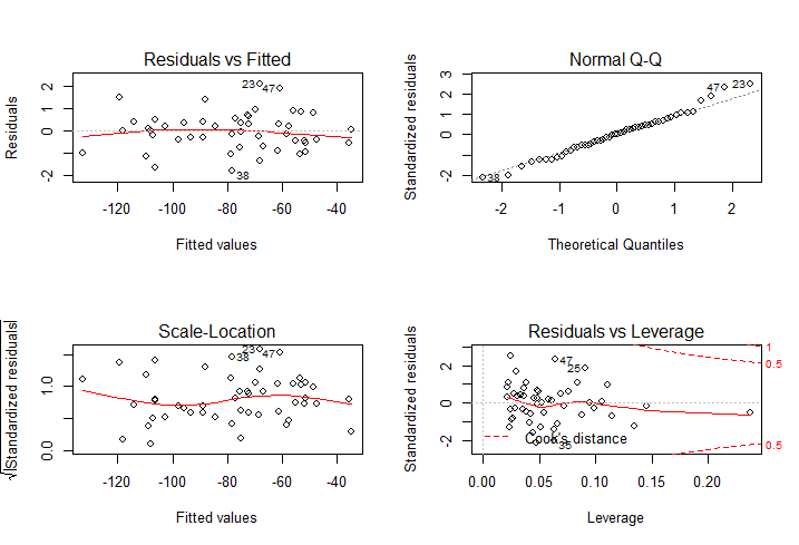 Figure 1 Regression diagnostics.
This model explains the most variance (r2 = 0.9988), and there is no significant violation of the assumptions of linear regression4, 5.
Generalized linear model
When the response variable is assumed to follow an exponential family distribution (binomial or poisson…) instead of a normal distribution (you can try to transform the data to normal distribution with a log-transformation or square-root transformation… first), the response variable is not a “linear” function of the predictors anymore. But we can use an arbitrary function (the link function) of the response variable to transform the nonlinearity to linearity6. I use a logistic regression as an example.
1
2
3
4
5
6
7
8
9
10
11
12
13
14
15
16
17
18
19
20
21
22
23
24
25
26
27
28
29
# A binary variable
y2 <- rep(c(1,0),each=25)
glm1 <- glm(y2~x1+x2, family=binomial()) # "family" describes the error
# distribution and link function
summary(glm1)
## Call:
## glm(formula = y2 ~ x1 + x2, family = binomial())
##
## Deviance Residuals:
## Min 1Q Median 3Q Max
## -1.6889 -1.0563 -0.1228 1.0992 1.7871
##
## Coefficients:
## Estimate Std. Error z value Pr(>|z|)
## (Intercept) -2.16640 1.72941 -1.253 0.2103
## x1 0.15499 0.09279 1.670 0.0949 .
## x2 0.01757 0.02833 0.620 0.5351
## ---
## Signif. codes: 0 ‘***’ 0.001 ‘**’ 0.01 ‘*’ 0.05 ‘.’ 0.1 ‘ ’ 1
##
## (Dispersion parameter for binomial family taken to be 1)
##
## Null deviance: 69.315 on 49 degrees of freedom
## Residual deviance: 65.890 on 47 degrees of freedom
## AIC: 71.89
##
## Number of Fisher Scoring iterations: 4
Residual deviance occupies a high proportion of null deviance, and “x1” and “x2” are not significant in this model, so this model is nearly meaningless. There are many ways to calculate different kinds of R-squareds, try the package rms or pscl.
I will add two models, Generalized linear mixed-effects model and Phylogenetic generalized least squares model which I use sometimes.
###1. Generalized linear mixed-effects model (GLMM) Yes, there is a linear mixed-effects model (LMM). Mixed model contains a fixed effects part and a random effects part. Suppose our observations are obtained from different groups, and these groups may be randomly sampled from the population we are interested in, but there may exist non-independence among the groups. The group becomes a random factor in this study7, 8.
GLMM is the extension of LMM, I will give a GLMM example in the framework of generalized linear model. See this for more details of fitting LMM using package lme4.
1
2
3
4
5
6
7
8
9
10
11
12
13
14
15
16
17
18
19
20
21
22
23
24
25
26
27
28
29
30
31
32
33
34
35
36
37
38
# A group variable
group <- gl(5,10,labels=LETTERS[1:5]) # five groups, ten
# observations per group
# I use package "lme4"
library(lme4)
# GLMM function. For LMM, use the function "lmer" instead
glmm1 <- glmer(y2~x1+x2+(1|group),family = binomial)
summary(glmm1)
## Generalized linear mixed model fit by maximum likelihood (Laplace
## Approximation) [glmerMod]
## Family: binomial ( logit )
## Formula: y2 ~ x1 + x2 + (1 | group)
##
## AIC BIC logLik deviance df.resid
## 32.8 40.4 -12.4 24.8 46
##
## Scaled residuals:
## Min 1Q Median 3Q Max
## -1.55130 -0.07671 -0.00101 0.04991 1.32409
##
## Random effects:
## Groups Name Variance Std.Dev.
## group (Intercept) 85.87 9.266
## Number of obs: 50, groups: group, 5
##
## Fixed effects:
## Estimate Std. Error z value Pr(>|z|)
## (Intercept) -8.67466 6.28065 -1.381 0.167
## x1 0.25855 0.19063 1.356 0.175
## x2 0.13280 0.08165 1.626 0.104
##
## Correlation of Fixed Effects:
## (Intr) x1
## x1 -0.413
## x2 -0.700 0.277
###2. Phylogenetic generalized least squares model (PGLS) PGLS fits a linear model, taking into account phylogenetic non-independence between observations9, 10. You need a phylogenetic tree first. I use the dataset shorebird in the package caper directly.
1
2
3
4
5
6
7
8
9
10
11
12
13
14
15
16
17
18
19
20
21
22
23
24
25
26
27
28
29
30
31
32
33
34
35
36
37
38
39
40
41
42
43
44
45
46
47
48
49
50
51
52
53
54
55
56
57
58
# Load packages
library(caper)
# Load tree and species traits
data(shorebird)
tre <- shorebird.tree # you can "read.tree"
df <- shorebird.data # you can "read.table"
# Combine the tree and the data frame of species traits
dataTree <- comparative.data(
phy=tre, # the phylogeny
data=df, # the data frame
names.col="Species", # names in the data frame that
# will be used to match the tip
# labels of the tree, default
# values are the row names
vcv=FALSE, # whether to include a
# variance covariance array
warn.dropped=TRUE # whether to warn when data
# or tips are dropped
)
# PGLS function
pgls1 <- pgls(
log(Egg.Mass)~log(M.Mass), # model formula
data=dataTree, # the "comparative.data" object
lambda='ML' # the branch length transformations are
# optimised using maximum likelihood
)
summary(pgls1)
## Call:
## pgls(formula = log(Egg.Mass) ~ log(M.Mass), data = dataTree,
## lambda = "ML")
##
## Residuals:
## Min 1Q Median 3Q Max
## -0.074057 -0.013712 0.007195 0.020826 0.071846
##
## Branch length transformations:
##
## kappa [Fix] : 1.000
## lambda [ ML] : 0.956
## lower bound : 0.000, p = < 2.22e-16
## upper bound : 1.000, p = 0.047331
## 95.0% CI : (0.867, 1.000)
## delta [Fix] : 1.000
##
## Coefficients:
## Estimate Std. Error t value Pr(>|t|)
## (Intercept) -0.486129 0.205686 -2.3635 0.02093 *
## log(M.Mass) 0.688645 0.032647 21.0937 < 2e-16 ***
## ---
## Signif. codes: 0 ‘***’ 0.001 ‘**’ 0.01 ‘*’ 0.05 ‘.’ 0.1 ‘ ’ 1
##
## Residual standard error: 0.02905 on 69 degrees of freedom
## Multiple R-squared: 0.8657, Adjusted R-squared: 0.8638
## F-statistic: 444.9 on 1 and 69 DF, p-value: < 2.2e-16
These functions are just in their simplest format, look through the help files and change the parameters for more suitable calculations. In addition, it will be better to understand statistical theories underlying these models.