Basic manipulations on phylogenetic tree with R
20 Jan 2016Phylogenetic relationship
As last post says species traits are more similar between relative pairs while less similar between distant pairs. We need some mathematical definitions of the relationship for further calculations. Phylogenetic tree can quantify the relationships between species in certain scale. In other words, the distance matrix of the species’ relationships was demonstrated in a form of a tree. There are many methods and tools to construct a tree under different assumptions with multiple algorithms, based on the sequences of DNA or amino acid or other distinguishable traits. Even better, many supertrees have been built suitably at the level of species.
There are some tutorials about the primary phylogenetic analyses in R (this, this, this and this). I will give my example.
Load data
It seems many trees are in the newick format, and this format is concise and easy-to-use. It is a structured data format that looks like,
1
2
# A fake tree in newick
((((Tip1:1,Tip2:1.5)Node1:2,Tip3:4)Node2:1,Tip4:3)Node3:1,Tip5:5)Node4;
Tip1 - Tip5: tip names of the phylogeny, Node1 - Node4: nodes of the tree, the numbers are the branch lengths of the tip or node to its immediate ancestor, taxa in parentheses are sharing same immediate ancestor.
They are also some other formats like nexus, phylip… You can load or transform the data format to R easily.
Let’s see our tree.
1
2
3
4
5
6
7
8
9
10
11
12
13
14
15
16
17
18
19
20
21
22
23
24
25
26
27
28
library(ape)
# Read tree file. You can use a specified file
# (like "mytree.tre") loading it with
# "read.tree(file='mytree.tre')".
# Here I use a different way.
tre <- read.tree(text="((((Tip1:1,Tip2:1.5)Node1:2,Tip3:4)
Node2:1,Tip4:3)Node3:1,Tip5:5)Node4;")
# Simple figure, see Fig. 1
par(mfrow=c(1,2))
plot(tre)
title("1. A fake tree")
# Lengths of the branches
tre$edge.length
## [1] 1.0 1.0 2.0 1.0 1.5 4.0 3.0 5.0
# Names of the tips
tre$tip.label
## [1] "Tip1" "Tip2" "Tip3" "Tip4" "Tip5"
# Number of internal nodes
tre$Nnode
## [1] 4
# Names of the nodes
tre$node.label
## [1] "Node4" "Node3" "Node2" "Node1"
Change tips
Sometimes the tip labels (most time they are species names) in the tree are not consistent with the names in your dataset. You can change the names as follows.
1
2
3
4
5
6
7
8
9
10
11
12
13
14
15
16
17
18
19
20
21
22
23
24
25
26
27
# Function for substitution of the tip labels
sub_tip <- function (tree, labels, sub = T) {
# labels: a data frame, containing the labels in the
# tree and corresponding new labels.
# This function is just an example, there is a lot of space
# to improve it if you need more features.
if (sub) {
matched_tip<-tapply(tree$tip.label,1:length(tree$tip.label),
function(x) labels[which(labels$tree_label == x), "new_label"])
tree$tip.label<-as.data.frame(matched_tip)[,1]
}
return (tree)
}
# Assume we need change the tip labels
labels <- read.table(text="tree_label new_label
Tip1 A
Tip2 Tip2
Tip3 Tip3
Tip4 d
Tip5 Tip5
", stringsAsFactors=F, header=T)
tre <- sub_tip(tre,labels)
plot(tre) # see Fig.1
title("2. A renamed tree")
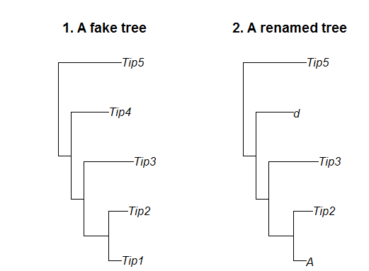 Figure 1 Two phylogenetic trees.
Combine and prune trees
1
2
3
4
5
6
7
8
9
10
11
12
13
14
15
16
17
18
19
20
21
22
23
24
25
26
27
28
29
30
31
32
# Combine two trees
# Another fake tree
tre2 <- read.tree(text="(((Tip6:1,Tip7:1.5)Node5:2,(Tip8:2,
Tip9:1)Node6:1.5)Node7:1,Tip10:4)Node8;")
par(mfrow=c(2,2))
plot(tre2) # see Fig.2
title("1. Another fake tree")
# Add "tre2" to "tre" at "Tip4"
# Notice that the lengths of the branches are the original values,
# make sure the two trees are additive.
treeCombine <- bind.tree(tre,tre2,where=4) # "where" is an integer giving the
# number of the node or tip of "tre"
plot(treeCombine) # see Fig. 2
title("2. The combined tree")
# Prune the tree
# Drop tips "Tip1", "Tip3" and "Tip4"
droppedTree <- drop.tip(treeCombine, c("Tip1","Tip3","Tip4"))
plot(droppedTree) # see Fig. 2
title("3. The tree after dropping tips")
# Extract the specific clade at "Node2"
extractedTree <- extract.clade(treeCombine, node="Node2")
plot(extractedTree) # see Fig. 2
title("4. The extracted tree")
par(mfrow=c(1,1))
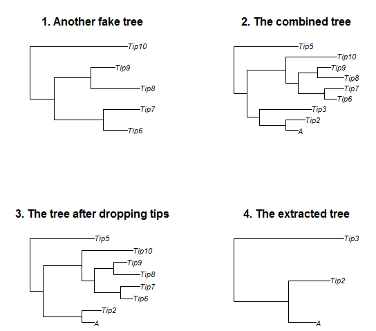 Figure 2 Four phylogenetic trees.
Plots
1
2
3
4
5
6
7
8
9
10
11
12
13
14
15
16
17
18
19
20
21
22
23
24
25
26
27
28
29
30
31
32
33
34
35
36
37
38
39
40
41
42
43
44
# I have not found better way to define colors for the branches,
# any suggestion?
cols <- rep("darkgrey",dim(treeCombine$edge)[1])
# A clade will be drawn in blue
range <- which(treeCombine$edge[,1]==12)
cols[seq(range[1],range[2])] <- "blue"
# Another clade will be drawn in red
range <- which(treeCombine$edge[,1]==14)
cols[seq(range[1],range[2])] <- "red"
# Width of the branches
wid <- cols
wid[] <- 1
wid[cols!="darkgrey"] <- 2
# Colors of the tip labels
tipCols <- rep("darkgrey",length(treeCombine$tip.label))
tipCols[treeCombine$tip.label %in% tre2$tip.label] <- "red"
tipCols[treeCombine$tip.label %in% extract.clade(tre,
node="Node2")$tip.label] <- "blue"
plot(treeCombine,
type="phylogram", # the type of tree, "cladogram",
# "unrooted", "radial" or any other type
show.tip.label=TRUE, # show the tip labels or not
show.node.label=FALSE, # show the node labels or not
edge.color=cols, # colors of the branches
edge.width=wid, # width of the branches
cex=0.8, # the size of the labels
direction="rightwards", # direction of the tree
tip.color=tipCols # colors used for the tip labels
)
# Label the node
nodelabels(c("A clade","Another clade"), # label
c(12,14), # node
frame="rect", # frame around the text,
# "rect", "circle" or "none"
col="darkgreen", # color
bg="yellow", # background color
cex=0.8
)
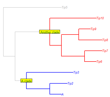 Figure 3 The phylogenetic tree.
You can make more interesting tree visualizations with package ggtree which is an extension of ggplot2. Click the figures below for details.

