Discriminant Analysis of Principal Components (DAPC)

DAPC

I should declare first that I am not good at molecular ecology. Recently I met a clustering issue which referred to amino acid sequences, and some newest papers point to using DAPC. It seems that DAPC becomes a standard method to define genetic clusters in this field (it can also be applied to other quantitative data). adegenet is a powerful package “devoted to the multivariate analysis of genetic markers data”. And I learn nearly everything from its tutorials hosted on GitHub.

Loading data

I know little about DNA extractions, amplification, genotyping…, so I will omit these steps. What I got is a cleaned data frame containing information about the individuals, “loci” (DNA or proteic sequences…) and “alleles” (alleles or amino acids…). I will use the data set nancycats in the package (which gives the microsatellites genotypes of 237 cats) as en example.

1
2
3
4
5
6
7
8
9
10
11
12
13
14
15
16
17
18
library(adegenet)
data(nancycats)

# "df" is the data form we always face to (at least for me) 
df <- nancycats$tab
class(df)
## [1] "matrix"

df[1:5,1:5] # individuals in rows, alleles in columns
##      fca8.117 fca8.119 fca8.121 fca8.123 fca8.127
## N215       NA       NA       NA       NA       NA
## N216       NA       NA       NA       NA       NA
## N217        0        0        0        0        0
## N218        0        0        0        0        0
## N219        0        0        0        0        0

# NAs replaced with zero (it is up to you)
df[is.na(df)] <- 0

Identifying clusters

We should define the groups (clusters) before doing DAPC. The function find.clusters can find the number of groups maximizing the variation between groups using k-means clustering algorithm. It is suggested that transform the data using a principal component analysis (PCA) before the clustering procedure, and this step is integrated in the function. Moreover, you can choose the optimal k (the number of clusters) based on the BIC (the default measure of goodness of fit) among a series of models coming from successive k-means with an increasing number of clusters. If you can not determine the number of retained PCs (using PCA) and the number of clusters before the analysis, you can run this function interactively with the fewest parameters. For how many clusters there are really in the data:

There is no longer a “true k”, but some values of k are better, more efficient summaries of the data than others…the actual number retained is merely a question of personal taste…

1
2
3
4
5
6
7
8
9
10
# Identify clusters using k-means interactively. 
# BICs here does not change so dramatically as the example 
# in the tutorial. I choose 3 clusters here.
grp <- find.clusters(df)
# Choose the number of PCs (Fig. 1), 100 here
## Choose the number PCs to retain (>=1): 
## 100
# Choose the number of clusters (Fig. 2), 3 here
## Choose the number of clusters (>=2:
## 3

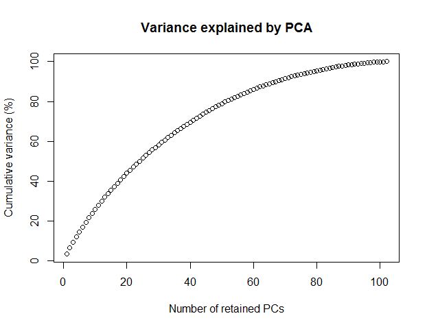Figure 1 Variance explained by PCA.

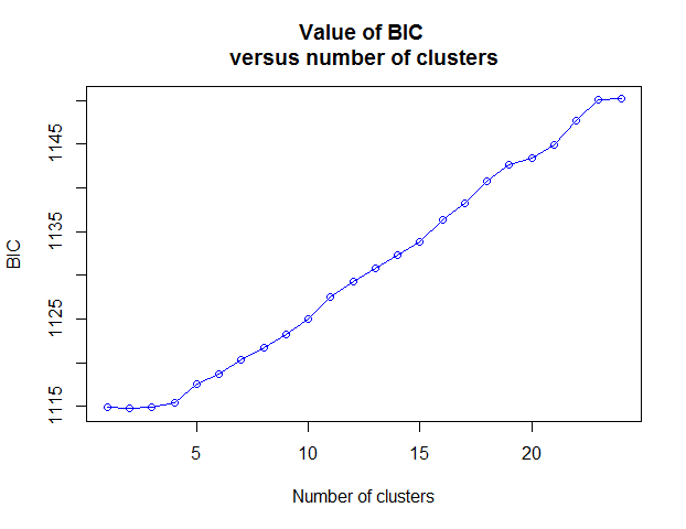Figure 2 Value of BIC versus number of clusters.

The DAPC

DAPC transforms the data using PCA, and then performs a discriminant analysis on the retained principal components. There should not be too many PCs for avoiding over-fitting to the specific individuals. This function is also interactive if no enough parameters were provided.

1
2
3
4
5
6
7
8
9
10
11
12
dapc1 <- dapc(df, grp$grp,scale=TRUE)
# Choose the number of PCs (same picture as Fig. 1), choose 60 here
## Choose the number PCs to retain (>=1): 
## 60
# Choose the number of discriminant functions (Fig. 3), 2 here
## Choose the number discriminant functions to retain (>=1): 
## 2

# Plot the output of the DAPC, with the discriminant 
# analysis eigenvalues and PAC eigenvalues in insets (Fig. 4)
scatter(dapc1,posi.da="topleft",bg="white",scree.pca=TRUE,
    posi.pca="bottomleft")

OK, three clusters, and see Fig. 4.

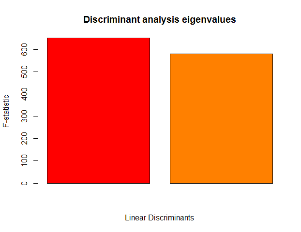Figure 3 Discriminant analysis eigenvalues.

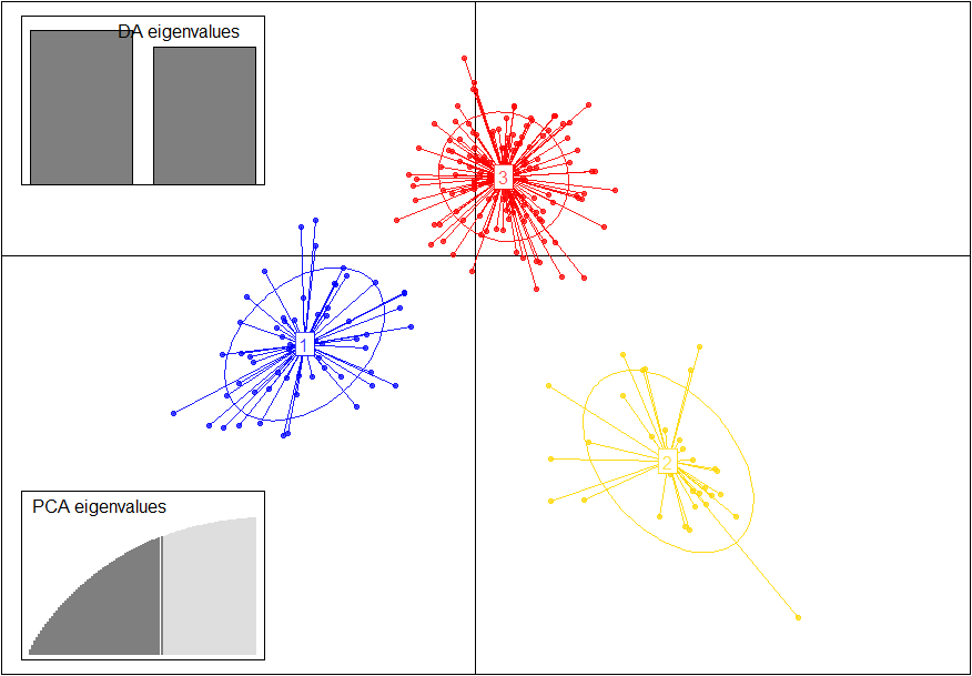Figure 4 Graphic outputs for Discriminant Analysis of Principal Components (DAPC).