Spatial Autocorrelation

Everything is related to everything else, but near things are more related than distant things.–Waldo Tobler^[1]

What is Spatial Autocorrelation (SA)?

As the first law of geography, SA is a measurement of the degree of similarity between spatial objects. A dependency exists between values of a variable in proximal locations. There are three kinds of SA: positive, negative and random (zero) (Fig. 1).

• Positive SA is when spatial data values tend to be clustered (similar values aggregate together in space).
• Negative SA is when spatial data values tend to be dispersed (dissimilar values cluster together).
• Random SA with no clear pattern.

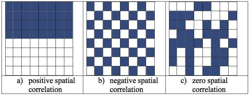Figure 1 Type of spatial autocorrelation^[2].

Most spatial data are clustered in ecology. For example, altitude values will always be relatively high near the peak of a mountain. Mean temperature will change smoothly from one place to another. Or there is a significant ecological pattern, but it will not be random. Many people treated SA as a useless parameter and excluded it in their studies when they want to using a spatial variable to reveal an ecological phenomenon. But the existence of SA will violate the independent observations assumption which is a precondition for many statistical methods. Positive dependence makes the effective sample size less than the number of observations. In many ecological examples, SA can arise from the focused variable or other factors that affect this variable. Moreover, positive autocorrelation can indicate different patterns at different scales (Fig. 2), that make it more complicated.

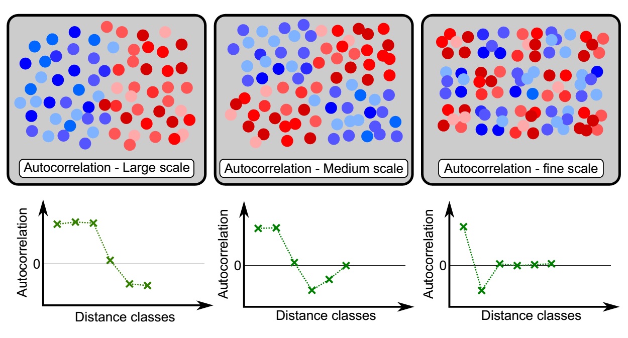Figure 2 Spatial autocorrelation at different scales^[3].

How can we detect SA in R?

We use the shapefile eire included in the package spdep as an example to test for SA. Let’s load the required packages and data firstly.

1
2
3
4
5
6
library(maptools)
library(rgdal)
library(spdep)

eire <- readShapePoly(system.file("etc/shapes/eire.shp", package="spdep")[1],
    ID="names", proj4string=CRS("+proj=utm +zone=30 +units=km"))

1. Build a neighbors list

1
2
3
4
5
eire.nb <- poly2nb(eire)

# Plot the spatial polygons and add the neighbors lists (Fig. 3)
plot(eire)
plot(eire.nb, coordinates(eire), add=TRUE, lwd=2, col='blue')

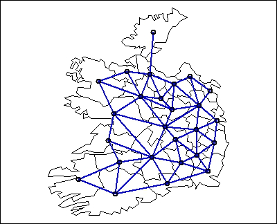Figure 3 Plot of neighbors list.

2. Create a spatial weights matrix for the neighbors lists

1
2
# Row-standardized weights matrix
eire.nb.w <- nb2listw(eire.nb)

3. Run statistical test to examine SA

We test SA of the variable A (percentage of sample with blood group A) in eire data sets.

Geary’s C

Computation of squared differences of values that are geographic neighbors, 0-1 for positive, 1 (expected value) for random and 1-2 for negative SA.

1
2
3
4
5
6
7
8
9
10
11
12
geary.test(eire$A,listw=eire.nb.w)

##     Geary's C test under randomisation 

## data:  eire$A 
## weights: eire.nb.w  

## Geary C statistic standard deviate = 4.5146, p-value = 3.172e-06
## alternative hypothesis: Expectation greater than statistic
## sample estimates:
## Geary C statistic       Expectation          Variance 
##        0.38011971        1.00000000        0.01885309     

Moran’s I

Computation of cross-products of mean-adjusted values that are geographic neighbors, -1 to nearly 0 for negative, -1/(n-1) for random and 0-1 for positive.

1
2
3
4
5
6
7
8
9
10
11
12
moran.test(eire$A,listw=eire.nb.w)

##     Moran's I test under randomisation

## data:  eire$A  
## weights: eire.nb.w  

## Moran I statistic standard deviate = 4.6851, p-value = 1.399e-06
## alternative hypothesis: greater
## sample estimates:
## Moran I statistic       Expectation          Variance 
##        0.55412382       -0.04000000        0.01608138 

Moran’s I and Geary’s C are inversely related. The results demonstrate that there is positive SA for variable A. But we should be cautious with the results because these tests are highly sensitive to the form of neighbors relationships, the choice of spatial weights and other factors.

References: